Significance- A false assumption?
Posted on April 3, 2024 • 6 minutes • 1266 words
“In God we trust. All others must bring data”, a famous quote often gives the impression that data is all powerful and this is what drives technology ahead. Dear readers, I am here to bust this myth on the importance and significance of data. My claim might sound preposterous, as we currently witness the data-driven technological rise. Not in this age, but data has always had significant value for human belief. Seers and thinkers of the past have always requested more data from even Gods to strengthen their beliefs. Shepherds collected data on their sheep to estimate their profits that year. Astronomers collected data on stars and kings on soldiers. It is true when people say data is power.
But wait, did I challenge this belief? Explorers! Let me ask you if you have beliefs that do not fit what the data suggests. You might believe people with glasses are smart, exercise increases your height, or sugar pills (or alternate medicine) cure diseases. Some of your beliefs are so true that you don’t just think they are, but you know they are. If data was all-powerful, should the data not suggest truth? Should data not be wrong?
In this blog post, let’s see what data truly suggests and how scientists try to make sense of it.
Data is all-pervasive and all-inclusive. Data can be both true and false, but the data that matters to scientists is the “Significant data”. Looking at the past weather data, one would find rainy days distributed across different seasons. You would only call it a Monsoon season if you find a “significant number” of rainy days during that season. To better understand the significance, one must better understand its opposite, randomness.
Consider an example where you would like to know your friend’s favourite ice cream flavour. If you find your friend often picks up the chocolate flavour, that would likely be his favourite. If this person does not have a preference, he would randomly pick up a flavour and you would never know the truth. Significance is something that tells you how different your friend is from being random. If he were to pick 100 times and he picks all four flavours 25 times each, you would say for sure that he does not have any favourites.
Now think about this. If he picks 37 times chocolate and other times the other flavours, would that tell you he has a liking for chocolate? Probably not. You could find this effect in approximately 6% even if these 100 pickings happened randomly. If you were to believe what many scientists believe, your friend has no preference for chocolate with the given data. I know this might sound strange but this is exactly what drives scientific understanding.
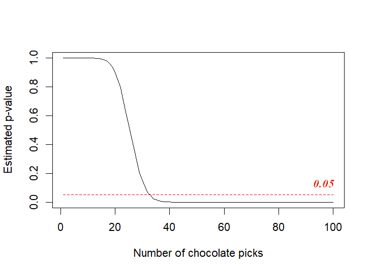 Significance is derived from understanding how different is the data from randomly generated data. In the above example, I randomly generated 10,000 scenarios where the probability of picking chocolate is 0.25 and in 6% of these cases, chocolate would be picked more than 37 times. This is called the p-value or the probability value. A p-value of 5% is often considered significant to believe the data to be true.
If you feel your brain releasing steam, then take a deep breath. There is more to “Significance” than what we just discussed. So far, we have seen that meaningful data has a low chance of random occurrence. In the abovementioned example, we also assume that our friend is sensible. Coz we all have that one poor friend who owns an iPhone. You could have a friend who always takes chocolate and another who rarely picks chocolate despite it being their favourite flavour. When we consider a normal distributed population, we have all types of people and the p-value we calculate might not tell the truth.
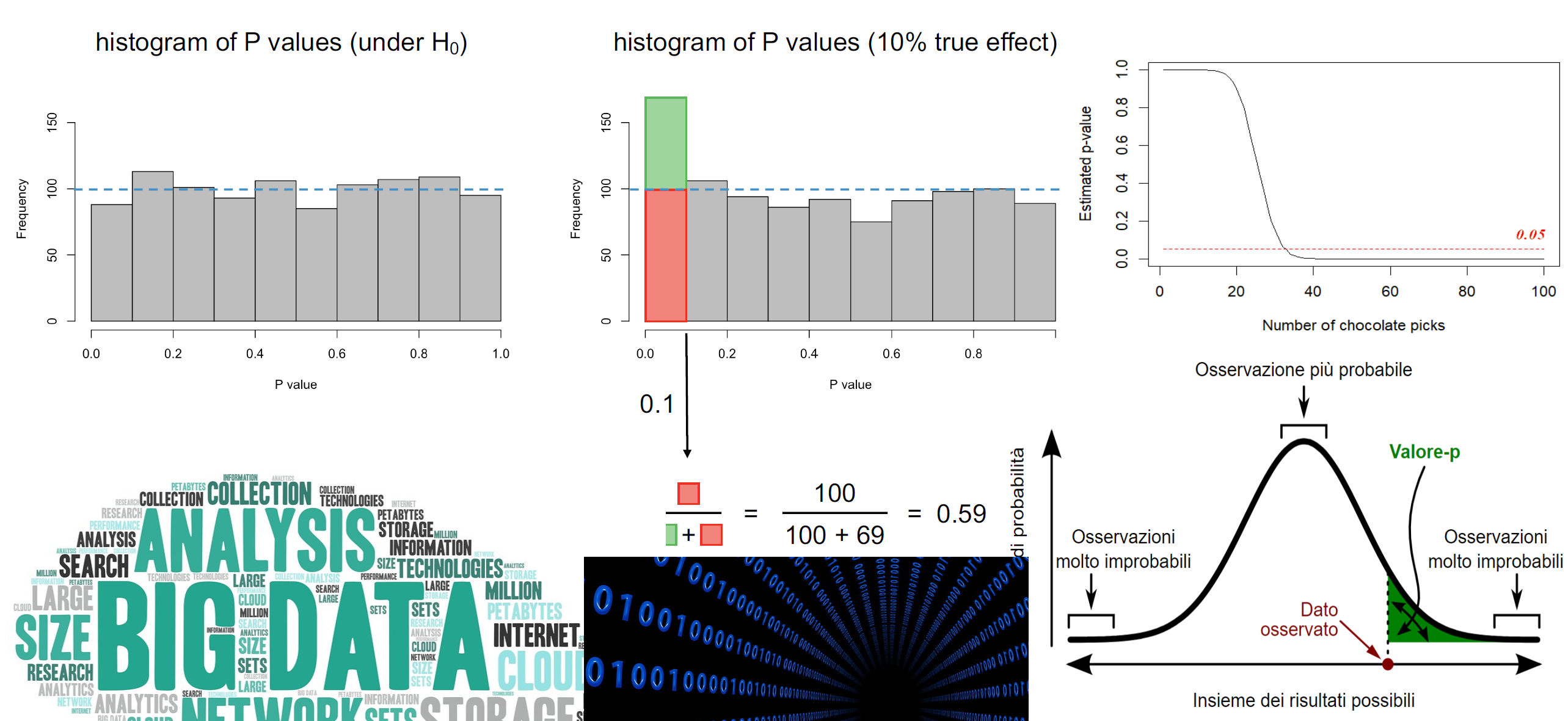
If we randomly pick values from a normal distribution and calculate p-values, we would have all p-values having equal probability of occurrence. This includes what we consider “significant” p-values. To put it in simpler terms, even if I blindfold a group of children and ask them to pick ice cream flavours, you could still calculate that 5% of children significantly “like” chocolate. Children here are blindfolded, so your conclusion is wrong. It is indeed random. I have below shown how all p-values have an equal likelihood of occurrence.
This is where the concept of FDR (False Discovery Rate) emerges. If in the population, there is indeed a significant phenomenon happening (children in general like chocolate), you should expect more “significant” p-values. Now that we know this, we can adjust the p-values to show what could be the true probability. Or can we? In the example of the below figure, “If we assume our occurrence has a 10% chance of happening by a random event, then only 59% of such occurrences are significant”.
Significance is derived from understanding how different is the data from randomly generated data. In the above example, I randomly generated 10,000 scenarios where the probability of picking chocolate is 0.25 and in 6% of these cases, chocolate would be picked more than 37 times. This is called the p-value or the probability value. A p-value of 5% is often considered significant to believe the data to be true.
If you feel your brain releasing steam, then take a deep breath. There is more to “Significance” than what we just discussed. So far, we have seen that meaningful data has a low chance of random occurrence. In the abovementioned example, we also assume that our friend is sensible. Coz we all have that one poor friend who owns an iPhone. You could have a friend who always takes chocolate and another who rarely picks chocolate despite it being their favourite flavour. When we consider a normal distributed population, we have all types of people and the p-value we calculate might not tell the truth.
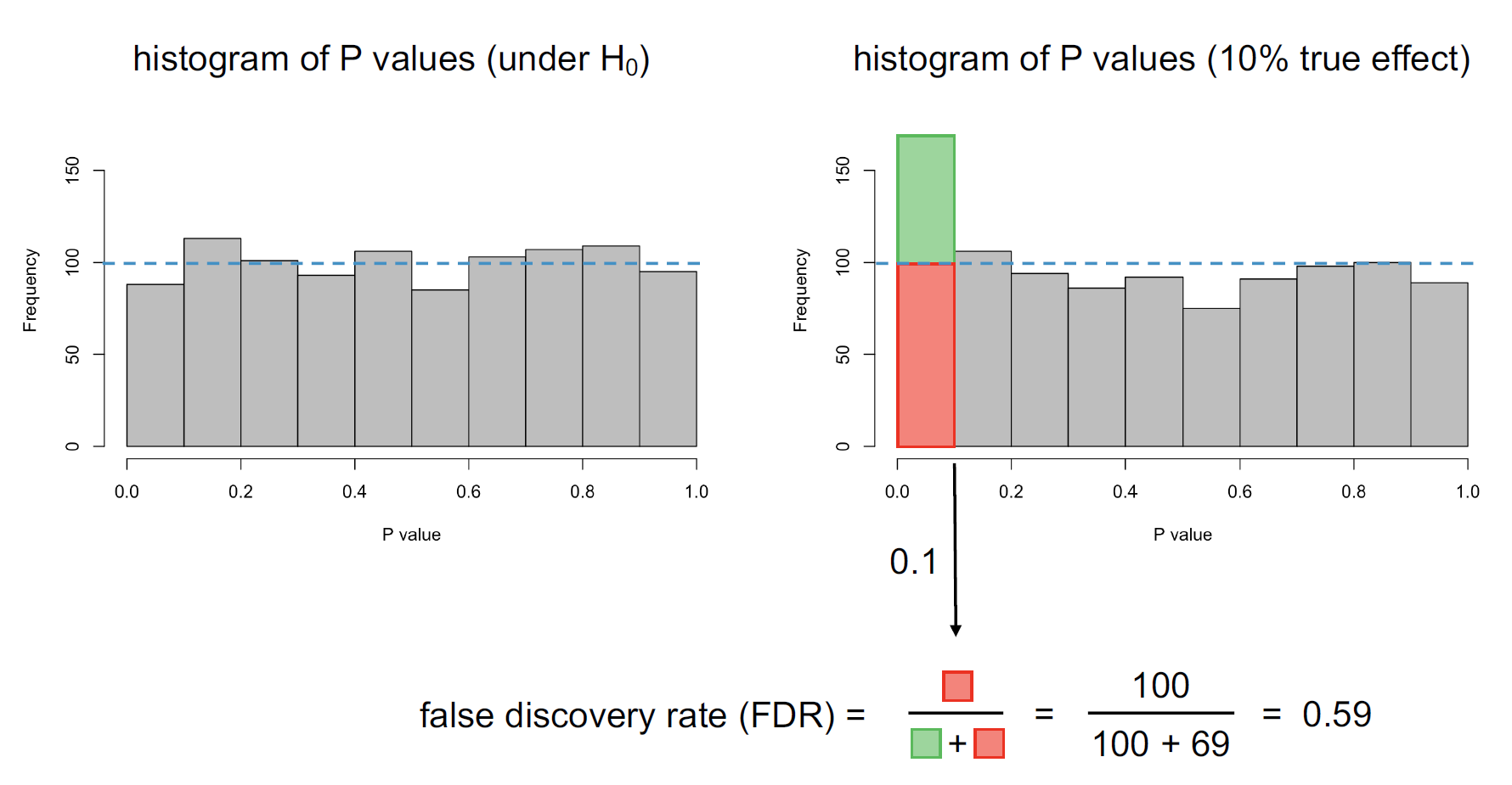
If we randomly pick values from a normal distribution and calculate p-values, we would have all p-values having equal probability of occurrence. This includes what we consider “significant” p-values. To put it in simpler terms, even if I blindfold a group of children and ask them to pick ice cream flavours, you could still calculate that 5% of children significantly “like” chocolate. Children here are blindfolded, so your conclusion is wrong. It is indeed random. I have below shown how all p-values have an equal likelihood of occurrence.
This is where the concept of FDR (False Discovery Rate) emerges. If in the population, there is indeed a significant phenomenon happening (children in general like chocolate), you should expect more “significant” p-values. Now that we know this, we can adjust the p-values to show what could be the true probability. Or can we? In the example of the below figure, “If we assume our occurrence has a 10% chance of happening by a random event, then only 59% of such occurrences are significant”.
 It must be noted that FRD is a population representation and the adjusted p-values only make sense if the population is very large. If we have less data, we might tend to assume many events as “significant” which might not be the case.
While we manage to understand how randomness has a great potential to show a “significant” occurrence, it is hard to discriminate between a true occurrence from a random occurrence. This thought leads me to self-enquiry. Could I ever understand whether the events that led me to where I am were significant occurrences or just random? I know deriving meaning from my experiences could be a foolish thing to do and so does ignoring my belief in significant events. All we can do is embrace all the events that happened to us and go ahead with a smile. For reality is always hidden in the veil of randomness. Or is it?
I have below attached the R code that was used if you would like to replicate it.
# Function to simulate ice cream picking
simulate_ice_cream <- function(n_picks, n_chocolate, n_simulations = 10000) {
  # Probability of picking chocolate
  p_chocolate <- 1/4

  # Simulate n_simulations ice cream pickings
  successes <- 0
  for (i in 1:n_simulations) {
    picks <- sample(c("chocolate", "other"), size = n_picks, replace = TRUE, prob = c(p_chocolate, 1 - p_chocolate))
    if (sum(picks == "chocolate") >= n_chocolate) {
      successes <- successes + 1
    }
  }

  # Calculate p-value (proportion of successes)
  p_value <- successes / n_simulations
  return(p_value)
}

# Set number of picks and desired chocolate picks
n_picks <- 100
n_chocolate <- 30

# Run simulation and print p-value
perct <- simulate_ice_cream(n_picks, n_chocolate)
cat("Percent of picking at least", n_chocolate, "chocolate times in", n_picks, "picks:", perct, "\n")
cat("Estimated two_tailed p-value:", 2 * min(perct, 1 - perct))
#draw a graph between different x values and estimated two_tailed p-value
x <- seq(1, 100, 1)
y <- sapply(x, function(x) simulate_ice_cream(n_picks, x))
plot(x, y, type = "l", xlab = "Number of chocolate picks", ylab = "Estimated p-value")
lines(x, rep(0.05,100), col = "red", lty = 2)
y[37]

#Generate random x and y normal distributed numbers and compare significance with t-test
x <- rnorm(100, mean = 0, sd = 1)
y <- rnorm(100, mean = 0, sd = 1)
t.test(x, y)$p.value # 0.2653
for (i in 1:1000) {
x <- rnorm(100, mean = 0)
y <- rnorm(100, mean = 0)
pvals[i] <- t.test(x, y)$p.value
}
mean(pvals <= 0.1) # 0.088 (~0.1)
padj <- p.adjust(pvals, method = "fdr")
mean(padj <= 0.1) # 0
y.mu <- rep(c(0, 0.4), c(900, 100))
for (i in 1:1000) {
x <- rnorm(100, mean = 0)
y <- rnorm(100, mean = y.mu[i])
pvals[i] <- t.test(x, y)$p.value
}
mean(pvals <= 0.1) # 0.169
padj <- p.adjust(pvals, method = "fdr")
mean(padj <= 0.1) # 0.067